Livak Method (Livak & Schmittgen, 2001)

Noga Mano | Research Methods B | June 2026

Introduction:

The Necessity of Post-qPCR Data Analysis:

Following a qPCR run analyzing gene reactions for stressors or inhibitors, we obtain outputs raw Cycle Threshold (C_t) values. These values reflect initial cDNA transcript abundance, but they cannot be directly compared or interpreted biologically, due to inherent experimental variations.

To extract meaningful scientific insights, processing raw data through the calculation method is essential for understanding the gene reaction under stress conditions, compare to normal conditions.

Post-qPCR mathematical processing is required to eliminate technical-background “noises”, establish a relative baseline and translate exponential data into true biological trends.

Preliminary Step: Experimental Setup & Gene Selection

Targeted Genes Defining:

Define your target gene(s) of interest and a stable internal reference (housekeeping) gene:

:memo: Reference (housekeeping) gene: a stable gene which the known stressor/factor we chose to check will not effect it.

:memo: Target gene: gene or genes that we expect to react upon known stressor/factor.

Experimental Design:

Design and conduct a controlled experiment consisting of:

:memo: Experimental/Treatment Group: Exposed to the specific stressor/inhibitor.

:memo: Control Group: Keep under unstressed conditions.

Quantification:

Perform quantitative PCR (qPCR) to obtain raw cycle threshold (C_t) values for all samples.

Arrange the result of the qPCR in table:

Table 1: Cycle Threshold (C_t) - an example

Treatment	Tubulin1	ascs	Delta	ets	foxA	gcm	NGN	opt	pak3	pak4	pitx	SM30	sm50	soxC	synB
DMSO Control	23.30	29.09	25.96	24.72	24.37	28.35	28.35	31.02	25.41	25.57	29.68	20.97	23.70	25.07	24.13
Inhibitor treatment	23.30	28.51	25.54	24.44	23.72	28.18	27.35	31.71	25.29	25.25	31.72	21.77	24.81	24.33	24.06

¹ Reference gene

Step 1: Internal Data Normalization (ΔC_t)

Normalize the target gene expression against the internal reference gene to account for variations in initial cDNA template concentration.

Minor variations in RNA quality, reverse transcription efficiency and/or pipetting are inevitable. Subtracting the Ct values of a stable reference gene (e.g., Tubulin) from the target gene controls for these confounding factors, ensuring that observed differences reflect true biological responses rather than technical artifacts.

Calculated Parameter: ΔC_t

Formula:

\[\Delta Ct = Ct_{\text{target}} - Ct_{\text{reference}}\]

Example:

Tubulin DMSO Control = 23.30

ascs DMSO Control = 29.09

DMSO Control (Δ𝐶𝑡) = 29.09 - 23.30 = 5.798

Tubulin Inhibtior treatment = 23.30 (the right reference gene - no change under stress treatment)

ascs Inhibtior treatment = 28.51 (a clear difference between control and stress treatment)

Inhibtior treatment (Δ𝐶𝑡) = 28.51 - 23.30 = 5.213

As shown in the table 2:

Table 2: ΔCt calculation

Treatment	Tubulin	ascs	Delta	ets	foxA	gcm	NGN	opt	pak3	pak4	pitx	SM30	sm50	soxC	synB
DMSO Control ΔCt	0.000	5.798	2.668	1.421	1.070	5.059	5.056	7.725	2.110	2.276	6.383	-2.327	0.405	1.777	0.831
Inhibtior treatment ΔCt	0.000	5.213	2.242	1.142	0.427	4.883	4.057	8.413	1.999	1.957	8.429	-1.529	1.515	1.032	0.764

Step 2: Normalization to the Control Group (ΔΔCt)

Calculate the relative change of the target gene within the stress treatment group compared to its baseline expression in the control group.

Baseline Comparison (ΔΔCt): Gene expression changes are relative. Subtracting the baseline expression of the control group (e.g., DMSO control) from the experimental group, isolates the net effect of the treatment.

Calculated Parameter: ΔΔCt

Formula:

\[\Delta\Delta Ct = \Delta Ct_{\text{experimental}} - \Delta Ct_{\text{control}}\]

Note: Typically, the average ΔCt of the control group is subtracted from each individual sample’s ΔCt.

Example

ascs gene:

DMSO Control (Δ𝐶𝑡) = 5.798

Inhibtior treartment (Δ𝐶𝑡) = 5.213

ΔΔ𝐶𝑡 = 5.213 - 5.798 = -0.585

As shown in table 3:

Table 3: ΔΔCt calculation

Parameter	Tubulin	ascs	Delta	ets	foxA	gcm	NGN	opt	pak3	pak4	pitx	SM30	sm50	soxC	synB
ΔΔCt	0.000	-0.585	-0.426	-0.279	-0.643	-0.176	-0.998	0.688	-0.111	-0.319	2.046	0.798	1.111	-0.744	-0.067

Step 3: Calculation of Relative Expression = Fold Change

Convert the logarithmic ΔΔCt value into a linear value representing the exponential amplification of the PCR process.

Because PCR amplification is exponential, C_t values exist on a logarithmic scale (where a difference of 1 cycle represents a 2-fold change). Utilizing the $2^{-ΔΔCt}$ equation transforms these values into a linear Fold Change scale, providing an intuitive, publishable measure of gene upregulation or downregulation.

Calculated Parameter: Fold Change (Relative mRNA Expression)

Formula:

\[\text{Fold Change} = 2^{-\Delta\Delta Ct}\]

Example

ascs gene fold change:

ΔΔCt = -0.585

Fold change = 2^(-0.585) = 1.50

As shown in table 4:

Table 3: Fold change calculation

Parameter	Tubulin	ascs	Delta	ets	foxA	gcm	NGN	opt	pak3	pak4	pitx	SM30	sm50	soxC	synB
Fold change	1.00	1.50	1.34	1.21	1.56	1.13	2.00	0.62	1.08	1.25	0.24	0.58	0.46	1.68	1.05

Step 4: Data Visualization and Biological Interpretation

Generate a graphical representation (e.g., a bar chart) displaying gene expression levels under the tested stress condition. (X-axis: Experimental Groups [targeted genes]; Y-axis: Fold Change).

Graph 1: Fold change results

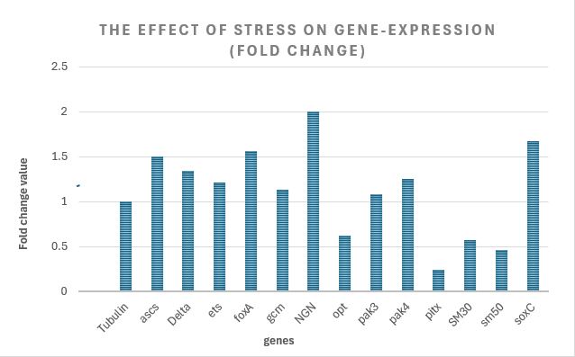
Looking at the bar chart, you can see which genes were upregulated / downregulated:

Fold change = 1 : inhibitor / stress have no effect on gene expression. Reference gene’s fold change should be = 1.

Fold change > 1 : gene expression increased (upregulated) under stress compared to the control.

Fold change < 1 : gene expression decreased (downregulated) under stress compared to the control.